TRADERS - Sizing Positions - Part 1

Published on Chartmill with kind permission of TRADERS’ Magazine. Check the original PDF article here

Trading and investing is simple, very simple actually. Particularly in financial markets. Because all we can do there, is just buy and sell stuff. Yet at this very basic level of making decisions, things already start to go awfully wrong. So however simple it may be, it sure isn’t easy. In this article we explain the single most important formula any trader and investor should know. In fact, it’s probably the only formula everyone should know about in life. And we’ll discover how most people who know the formula already, probably interpret and apply it the wrong way. Finally we’ll get into how to exploit all this and work the numbers.

If buying and selling is the only thing we can do, it has to be the only thing we can do wrong. And if problems start to emerge from those basic actions, we’d better look into them carefully. Any transaction in financial markets is the consequence of orders being executed. When we take a closer look at any order, we always have to include at least three types of information:

• whether we want to buy or sell, or plainly direction
• what we want to buy or sell, mostly addressed as selection
• how much we want to buy or sell, let’s call this sizing

Next to that, of course, we have to decide when we want to buy or sell. This is called timing. Timing can be explicit, when timing information is provided within the (conditional) order, or implicit, when timing is done by actually placing the order for immediate execution, in which case ‘when’ gets narrowed down to ‘now’.

This leaves us with four main dimensions: direction, selection, timing and sizing. In this article we are going to have a good hard look at what dimension might be most important to trading. In the following articles of this series, we are going to quantify everything in a practical way.

There’s a bit of calculus in the next section. But it all comes down to the basic operations of addition, subtraction, multiplication and division. So stay with us, it definitely will be worth your while.

On the origin of profits

Where does a net profit or loss come from? If we can answer that, maybe we will have a better shot at obtaining the first and avoiding the latter. Let’s take a case at hand. Suppose we have the following profits and losses:

This makes for a total net profit of 2. We’re using small and whole numbers here, for the sake of simplicity. But any numbers could be used without compromising what will be derived from it. The first thing we’ll do is order the sequence and separate winners and losers. Of course, changing order won’t have any impact on the net result at all. When we do this we get:

Next we will multiply and divide the sum of profits by 4, which again keeps things neutral as to the net profit. We’re merely rearranging things at this moment. We’ll do the same for the group of losses with the number 6.

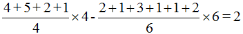
In case you wondered where the 4 and 6 come from, and you hadn’t figured it out yourself already, 4 is the number of winners, while 6 being the total number of losses. Now we can calculate any part of this equation without changing anything to its net result.

By doing this we get the values 3 and -1.67, 3 being the average profit of all winners, -1.67 the average loss of all losers. Finally lets divide everything by 6+4, the total number of trades.

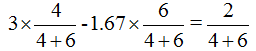
Simplifying things a bit, gets us

In this final form, it’s very clear we have 4 out of 10 trades giving us an average profit of 3, while 6 out of 10 trades have cost us 1.67 on average. Of course the net value doesn’t equal the total net profit of 2 anymore, since it also got divided by 10. Hence we have, on the right side of the equation 0.2, being the average net profit per trade.

What we have here is, in effect, a condensed way of summarizing profits and losses. But it’s far more than that. This formula was originally proposed by Blaise Pascal some 400 years ago as expectation or expectancy.

In a more general form we can write it down as:

Or fully:

Average result per trade = frequency of winners x average profit per winner - frequency of losers x average loss per loser

Expectancy dissection

So. We got some news for you. Question is, do you want it sugar coated or right between the eyes? Every trader who’s been around for a while or read at least a few books on the subject will probably be familiar with expectancy in some way or the other. But here’s the catch. It’s useless.

At least as far as the numbers are concerned. Popular trading theory has it that one only has to put in the numbers to see if a system or approach will be profitable, i.e. show a net average profit per trade. Having a positive outcome in your expectancy has become so important in research and backtesting they even gave it a name of its own. Referring to it as having an edge.

But any number we’re bound to put in is based on past trades. The frequency of winning and losing, as well as the average profit or loss, are only known in hindsight. We don’t know anything about the future and none of those figures have nor will be constant through time in an ever changing environment. What’s more, bounding any of these numbers to a period is absolutely necessary and therefore renders them useless, because an edge over a certain period can be there, while several smaller intervals within that same period can have a negative expectancy.

Beware of books and money management techniques that are based solely on the principle of meeting an edge by figuring out and building on historical expectancy. For one thing, it’s a formal fallacy called confirming the consequent or converse error. Those models may do a great job at greatly simplifying the problem at hand of understanding the importance of money management. However their simplification is artificially introduced and not a property of the reality they try to model. Besides evidence mounts that hardly any distribution in this context probably is statistically normal. What’s more, winners and losers have a tendency to cluster. Such clusters will coincide with periods of above and below zero expectancy. While expectancy may indicate a system as bad, clusters may point well towards the opposite. Good systems probably have a tendency for seeing their winners and losers cluster ^(*).

Bottom line, in trading any expectancy we calculate is a historical number as well and might give an analysis of the past. But it cannot be used for extrapolating the future.

Back to the drawing board?

So, out goes the expectancy formula, right? Well, not entirely. There are quite some important messages to take away from expectancy, at least that is, if you just look at it from the right angle.

Consider figure 1, where we visually depicted the example’s final state. In this picture we placed the average profit and loss as weights on equilibrium scales. Mind the subtle difference in the length of the scales’ arms, being proportional to the frequency of winners and losers. This picture sets the stage for more insight in the highly important concept of position size.

In this visualization of the expectation formula, two aspects become obvious. Represented by the weights and the arms of the scales, we have the size of the average profit and loss on the one hand and the frequency of winners and losers on the other.

The frequency of winners and losers is actually only one degree of freedom instead of two, because they complement each other. So we can define both with one number, typically called reliability. If you’d happen to have 100% winners, there would have to be zero losers and this would correspond with the utmost reliability. The other factor, average size of profits and losses, can also be compressed into one number most often identified as the profit/loss ratio or P/L ratio for short.

If we go back to the example, we have a reliability of 40%, which stand for 40% winners and consequentially 100-40 = 60% losers. The average winners has a profit of 3, while the average losers amounts to a loss of 1.67, indicating a P/L ratio of 3/1.67 = 1.80. This number indicates that, on average, 1.80 was made for every 1 that was lost. If these numbers would scale by ten, say to 30/16.67, the P/L factor would stay exactly the same, meaning the scales would keep the same balance, even though expectancy would rise tenfold.

Who’s in control

Focus here shouldn’t be on what all those numbers might be for the future, however nice to have they would be. The important question here is what part of the equation is most within our reach to control. Is it reliability or rather the profit/loss ratio?

Let’s take on reliability first. Do we have control over the number of winners and losers. Of course we all would love to have 100% winners. But that is, of course, impossible. For such a system would either throw financial markets out of action immediately or it would become a financial black hole attracting all the money in the end, also ending financial markets. So reliability must be somewhere between 0% and 100% winners, as figure 2 suggests. The effort needed to increase reliability is what we call analysis (also in determining direction). Pure fundamental analysis or technical analysis, despite heavy discussion among their prophets, are nothing more than different extremes on both end of the same spectrum, manipulating numbers from the past. With new numerical material becoming available at different frequencies.

But the truth is, analysis only gets us so far. Because the relationship between analysis effort and reliability, appears to be a power law. This means that the effort to take us from 30% to 40% winners, probably could have to be doubled or tripled to take us from 40% to 50%. The closer we to a 100%, the harder (exponentially harder) it will be, in terms of analysis effort (money, energy, time, …), to get even closer.

So while analysis can be worthwhile, people probably already do far too much of it. The problem is threefold. First, we are evolutionary tuned for wanting to be right. Being right implies having control. Having control over your environment or being able to anticipate on it, gives a firm edge in evolutionary terms. Secondly, because traders and investors are looking for certainty in an uncertain environment over which they have no control, they crave the illusion of control. Doing more analysis certainly gives this illusion, if not the control. Thirdly, general opinion has it that doing too much analysis cannot hurt. I beg to differ. Why not? Notice the dotted line on figure 2. Is it possible to obtain 100% losers by doing more analysis? If 100% winners is not reachable, why should 100% losers be reachable?

The proof is in the pudding as the amount of ads aiming on system reliability shows my hypothesis right. If we wouldn't bother too much about setups and analysis, but more on handling trades the right way once we have them, then ads wouldn't pay for themselves and we would stop seeing them. It’s a demand driven supply.

Another indication that focus is way too much on analysis is the alarming amount of information we try to digest and the speed at which we try to do so. It’s a losing game for a trader trying to beat the system by evermore analysis of evermore data on evermore smaller and smaller time frames. Instead we should zoom out and aim for even fewer but even bigger winners.

What we are trying to say here is not that analysis is useless and shouldn’t be done at all. But given the marginal added value at a certain point, we should aim at ‘just enough’. Given the 80/20 power law, the minority of our analysis probably accounts for the majority of its effect on our number of winners ^(°). By the same 80/20 law and the concept of least resistance, profits for a minority will be paid by the losses of the majority. So you have a better than average chance of having more losers at any one time.

Along the same lines, it’s not so much that analysis is overrated, as it is about the fact that we have far more control over the other dimension of the equation: the profit loss factor.

We do have a lot of control over the average size of our profits and losses. Pure theoretically, if we sell every loser when it hits a 5% loss, our average loss can’t mathematically get any bigger than 5%. Just by selling, which can be done with the simple click of a mouse. Something that needs no analysis at all. It’s something that can even be automated through conditional orders and options.

Does this work?

Our pupils at www.monest.net (currently a Dutch website with a an English spin-off into www.chartmill.com) obtain a nice 10% a year, on average, while learning to trade and applying, in a disciplined way, the material explained in this article series. But what’s more is that they stick to the system by biting the bullet when facing, again on average, 60% losses among all trades. That can be painstakingly difficult for new members. But understanding expectancy keeps them aboard when the going gets though.

Next time …

… we go into how we can use and implement the high degree of control we have over expectancy, by using risk control and controlling the size of our positions. We’ll also learn how to quantify position size.

^(*) See my article series on equity curve analysis in March, April, June and July issues.

^(°) This 80/20 cause/effect is actually all around in trading and investing. The large profits of a minority are paid out of the losses of a majority. The majority of our profits come from the minority of our trades. And so on …

[FIGURE 1]

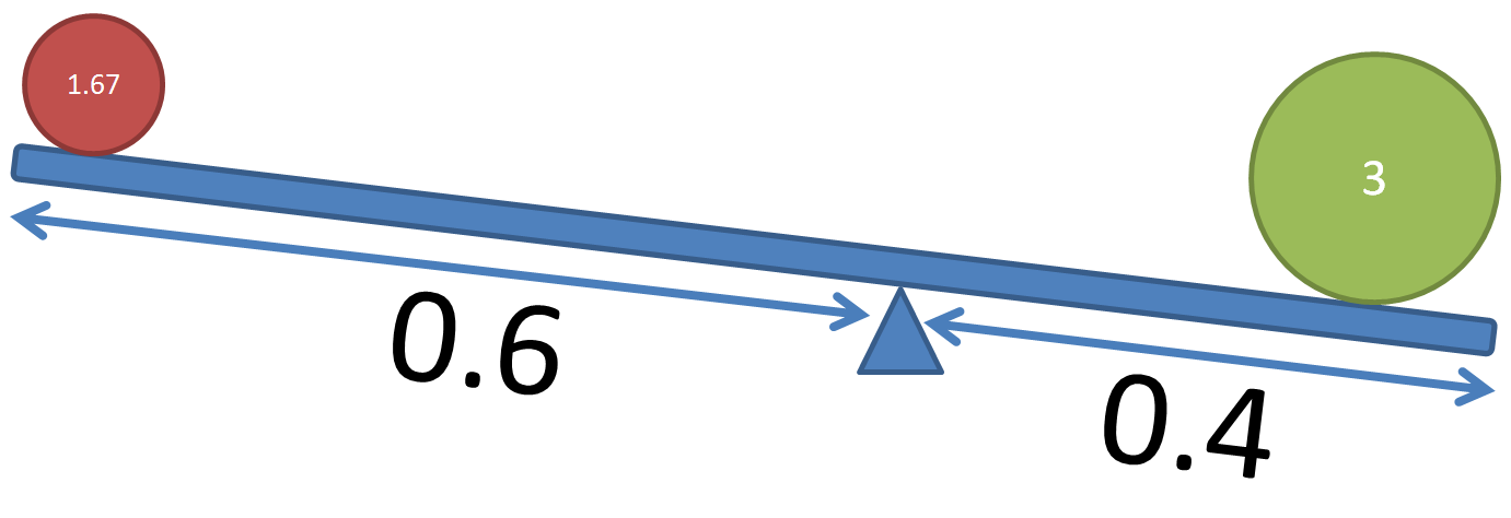
[HEAD] Expectancy equilibrium scales.

[CAPTION] Figure 1: On these scales the average profit (green) is balanced against the average loss (red). More importantly, the arms of the scales are proportional to the frequency of winners and losers. As such, in this example the average loss has a bit more moment of force than its counterpart on the other side. Nevertheless the frequency and average profit of winners makes up for the frequency and average loss of the losers. Resulting in a net profit.

[FIGURE 2]

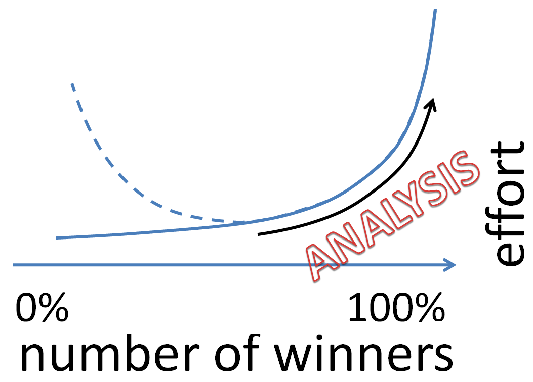
[HEAD] Analysis effort power law

[CAPTION] Figure 2: Behold doing too much analysis. The marginal effect of every bit of analysis we add to the picture, shrinks the higher our number of winners gets relatively to the number of users. So a successful system, as measured by its liability, has a natural resistance to becoming even better. Compare it to falling from the sky and reaching terminal velocity, the speed at which gravitational acceleration becomes balanced by air resistance. Or a boat’s sail catching more air resistance the faster the boat goes.

DIRK VANDYCKE is actively and independently studying the markets for over 15 year, with a focus on technical analysis, market dynamics and behavioral finance. He writes articles on a regular basis and develops software, which is partly available at his co-owned website www.chartmill.com. Holding master degrees in both Electronics  Engineering and Computer Science, he teaches software development and statistics at a Belgian University. He’s also an avid reader of anything he can get his hands on. He can be reached at dirk@monest.net.