TRADERS – Be(a)ware of diversification (part 2)

Published on Chartmill with kind permission of TRADERS’ Magazine. Check the original PDF article here

In the first article we decided to drag profits and total return into the picture of diversification, next to its common risk lowering incentive. This gave us a more realistic view on diversification. While the advantages on the risk side are clear to practically everyone, from the expert to the layman, we shifted focus to the disadvantages, mostly on the profit side. Diversification will spread risk, but to the cost of averaging returns. Let’s see if we can put this knowledge to our advantage while putting it in practice as well.

Diversification or concentration?

Expectancy, as depicted in figure 1, first of all, tells us that we have far more control over the average size of our winners and losers, than we have over their frequency, which is what all forms of analysis are all about. So instead of focusing on increasing the number of winners, whilst decreasing the number of losers, we should actually just try to minimize the size of losers and maximize the size of winners. So expectancy is the mathematical embodiment of the old trader’s adagio of cutting losses and riding winners.

Secondly, and of specific interest to us here, is the fact that this also implies that resources will have to flow from losers to ever fewer winners, eventually concentrating a portfolio rather than spreading it! For though it’s quite clear to most how to cut losses, i.e. by selling them early on, before the proverbial mistake becomes a problem, the answer to the question on how to maximize profits more often than not doesn’t get taken beyond holding on to winners. But winners can be added to as well, even accelerating the speed with winners get us more profits and as a consequence take a bigger piece of the portfolio pie.

Thirdly the mathematics of geometrical growth tells us the that diversification decreases the average return for sure. Take the example of having 9 winners of 1% and one winner of 25%. Average return in that case would be a mere or 3.18%, giving a total return of only 3.40%. If that wouldn’t be so or the effect would be negligible, that could only mean that the original returns must be very close to each other in which case diversification didn’t change a thing other than perhaps increasing transaction costs and again lowering return.

To look at this another way if diversification is contradictory to expectancy, concentration seems to the only valid option.

Of course all this raises the question if this doesn’t increase risk to unacceptable levels?  Let’s leave that question for later and first turn to experimental, well practical if you want, proof of all this. To address this I made use of a Monte Carlo simulation.

Or simulation?

The experiment I ran gave diversification the benefit of the doubt. I used a database of several tens of thousands of stocks (excluding low volume stocks, very low priced stock, non-regulated markets, overly volatile stocks and the like). Stock were monitored over several decennia, including a wide range of market conditions. My Monte Carlo simulator ran (and in the end averaged) several thousands of tests, each one going like this.

First a portfolio was made of thirteen randomly chosen stocks over a period specific to that test (I explain this in a moment). Initial capital was equally divided between all thirteen stocks. The computer than ran each portfolio in two copies. One copy was kept as a reference which I called the homogenous diversified portfolio. On might refer to this as an non-weighted index. The other copy did something very simple to get rid of the diversification and move over to the side of a concentrated portfolio gradually. This pruning-portfolio, as I named it, put a 3 ATR trailing stop underneath all positions. The trailing stop was of course only allowed to increase, as the general good practice ideas of using stops dictate. As soon as a position got stopped out, the cash would get distributed evenly over the existing holdings in the portfolio. Eventually only one stock would survive holding a hundred percent of the portfolio resources. As soon as this last one got stopped out, net return of both portfolios was captured. So the interval the reference portfolio got monitored depended on the moment the last stock of the pruning portfolio was stopped out. Hence a period ‘specific to the test’. From the thousands of tests that were run, some portfolio’s only lasted a few weeks while others took more than a year to get stopped out of their last holdings. So of course by now you must be wondering what the results of this experiment are. Here’s what I got.

Results are in

Take a look at the average return chart in figure 2. In there you have thirteen grey lines depicting the equity curves of all thirteen holdings in the pruning portfolio. As you will notice, some got drawn over a longer time interval than others, depending on how long they stayed in the portfolio. The un-interrupted black line is the equity curve of the pruning portfolio getting more and more concentrated, while the dashed black line shows the equity curve of the homogenously diversified reference portfolio. Keep in mind that these are averaged equity curves of the actual equity curves of thousands of tests run on samples of portfolios starting out with thirteen randomly chosen stocks.

Systematically concentrating funds in the winners/survivors, seems to be the better way. Which makes a great case for my warning against mindless diversification, i.e. without thinking things through first. Apart from giving a better end result on average, the return of the pruning portfolio stays on top of the diversified portfolio all along the way with a difference up to 2,36%, including transactional costs. And that’s even after realizing that in this setup the pruning portfolio has to make a lot of artificial costs just to un-spread itself. In reality a concentrated portfolio doesn’t have to start from a diversified one. Instead of having 13 round-trip costs as in the experiment, in reality a concentrated portfolio could be built up nicely in 3 to 4 entries and only one exit. That leaves room for up to 4 dips in the water (8 round-trips) and cutting the loss short, before starting to generate higher round-trip transaction costs than the homogenous diversified portfolio would leave you with.

But, but …

Isn’t that carelessly dangerous? After all, spreading did lower the average risk, right? Can you even imagine holding 180% of your portfolio (that also implies the use of margin already) in one position? No stop will protect you if it opens 40% lower on after-close news from the previous day.

Well the truth is, that never before in history have we been more able or have we had more tools at our disposal to fine-tune and isolate risk than at present. Going in depth through  all the tools and techniques available would take at least another article and probably a whole book. So let me just give an example in the above case of having, on margin, 180% of one’s portfolio into one stock. First of all, no one in his right mind would start out any position with 180% of his/her total capital. Such a position would only make its appearance after scaling in a stock that is appreciating. The scaling indeed accelerating the profits from the appreciation. So to begin with the position would already have to show quite a nice profit as the current stock price will probably would hold quite a distance from the average entry price. This would provide a first margin of safety. Of course if we don’t want to indulge in ‘mental accounting’, paper profits need to be cherished as much as initial capital or margined capital. A stop can take us already a long way but only so far. A simple technique to cope with this is to extract cash from the position by actually selling part or whole of the position, freeing up most of the cash and securing most of the profits, while exchanging a very small part of it for call options (in the case of a former long position). So instead of holding, say, 1000 shares worth $32,37 a piece, one could sell the shares, cashing them in for $32370 while buying 10 long to medium term call contracts for let say $3000 or only 9,27% of the original position. Cutting the downside to a fraction of what it was. No more than the option premium can be lost form there on. It’s like having a stop at 9,27% without having to worry about the whole thing gapping down. Next to cash extraction you can also use, what I call, volume extraction, trying to buy shares for the same amount at a lower price after selling on a new base breakout. By buying for an equal amount at a lower price, one can buy more shares without investing more capital in the position. Of course this will take more time to manage the portfolio.

So to take this home, instead of using diversification, pretty much the only thing available in earlier days to minimize risk, we should start using new ways of achieving this, without keeping on paying the negative consequences it brings with it.

[FIGURE 1]

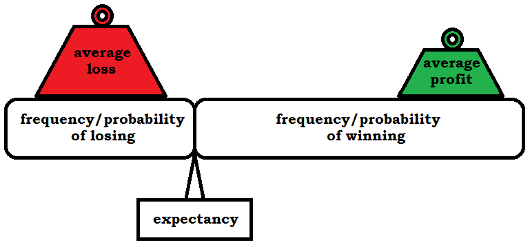
[HEAD] Expectancy depicted as scales.

[CAPTION] Figure 1: Being profitable in the long run with trading, and all investing for that matter, is about cutting losses and letting profits run. Although it’s a hearsay thing of ages, statistical expectancy actually proofs the saying mathematical. It’s not about being right or wrong but handling both profits and losses well.

[FIGURE 2]

[HEAD] Homogenous diversified portfolio versus a concentrated pruning.

[CAPTION] Figure 2: An average portfolio of thirteen randomly chosen stocks gets compared to its concentrated counterpart where the cash freed up by positions getting stopped out are divided amongst the survivors. The grey lines show the average returns from each individual (averaged stock) up until the point where they got stopped out. The black lines give the total return of both alternative portfolios.