TRADERS - Effective Volume: A Better Accumulation and Distribution Measure

Quite some research was already dedicated to the possible detection of accumulation and distribution processes in financial markets over the past decades. Nevertheless, the existing indicators aiming at defining and measuring accumulation and distribution are still susceptible to improvement. This article aims at explaining some of the most important revisions in that area and the resulting new (family of) indicators.

Let’s start off with having a look at the most widespread definition of accumulation and distribution. The most classic index there would probably be the one proposed by Larry Williams. Even though he suggested several improvements on his own later on, one of the most remarkable insights there came from our fellow Belgian trader Pascal Willain, as put forward in his book ‘Value in Time’, published by Wiley. But nevertheless we managed to still throw in some minor improvements ourselves at ChartMill. Let’s dig in.

A/D

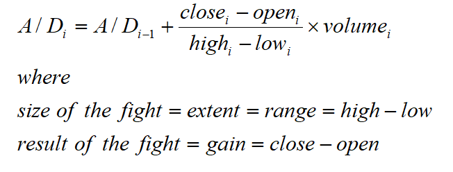
A common way to view accumulation and distribution is to look at the action in financial markets as a sport game or a battle between bulls (longs) and bears (shorts). In that action, we distinguish between the size and the outcome of the battle. Synonyms used for size here are the extent, or better yet, the range. The range over a certain interval, most often a day. It’s simply the difference between the highest price quoted during the interval and the lowest prices quoted. This will always be zero or greater (i.e. positive). In contrast, the outcome, also called the gain, is the difference between the interval’s opening and closing prices. Consequentially, this difference can be negative for an interval, when its close happens to be lower than its open. The classical ways to define accumulation and distribution all come down in some form of ratio between gain and extent. Some bring volume into the picture by multiplying the former ratio by it. The most popular accumulation distribution index is nothing more than a running sum of this ratio multiplied by volume or, as a formula:

Analyzing this formula in depth however, leads to various important shortcomings:

1. Most traders will agree that a close near the high is far better than a close near the low, something the above formula doesn’t account for.
2. Known to a lesser extent, is the fact that the opening price is more vulnerable to manipulation than is the closing price. Also, the opening price is highly influenced by overnight orders. Orders put in after the market close, the evening before or during the weekend.
3. Time redistribution of volume. The fact that volume distribution throughout the interval is regarded as being uniform. The larger the interval under study, however, the less such an implication keeps holding true and the bigger the error being made in estimating true accumulation and distribution. Even for the day-interval, volume is far from uniformly distributed (but rather U-shaped). For small intervals (e.g. one minute) this effect would be not to say inexistent.
4. Price redistribution of volume. Analogously to time redistribution of volume, most indicators reckon every price in an interval being equally weighted in all transactions over the interval. But of course also this might implicate quite an error being made on intervals as small as one day.
5. The formula doesn’t account for (opening) gaps. But gaps, if they appear, are part of the extent and gain for an interval. And a quite substantial part at that, sometimes.

Effective Volume

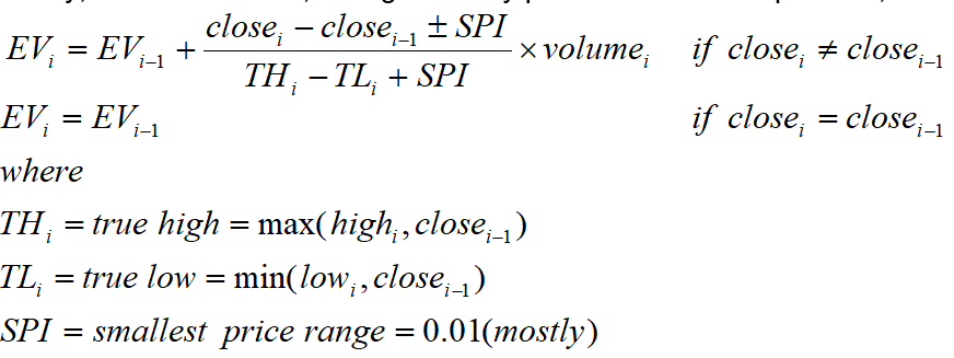
Trying to work away price and time redistribution of volume to begin with means using the actual volumes at the time and price they’re transacted. As such we have to stop using the EOD or interval data (i.e. open, high, low close and volume) that most indicators use today. To keep the of tick-by-tick data manageable, we can revert to minute intervals. That way errors, if any, are made are almost irrelevant due to the very small nature of the intervals. As luck would have it, by solving problems 3 and 4, in that way, we also take away problem 1. Because, again to due to the nature of the very small intervals, given enough liquidity, open, high, low and close for a single minute will almost always be very close to each other. Mind the fact that if that wouldn’t be the case, we could further decrease the intervals or use actual tick-data. Leaving us with two problems, both can be addressed by exchanging the opening price openi in the formula for the previous interval’s close closei-1. That way gaps are included in the formula, while easy to manipulate opening prices are out of the picture. Nevertheless this doesn’t take away problem 5 entirely, because gaps are not accounted for in the denominator of the formula. To do just that we replace the high and low for the interval by the true high and true low. According to those definitions, when having a gap down, the previous close would be the current interval’s high. Likewise, in the presence of a gap up, the previous close would serve as the current interval’s low. That way, the true high of an interval is the maximum of the previous interval’s close and the high of that interval, while the true low would be the minimum of the previous interval’s close and the current interval’s low. One last fix is due to price count in an interval. Imagine the minute interval having a range between, let’s say, 2.34 and 2.37. That range would normally be calculated as the difference between those numbers, being, in this case 0.03. However, there are four, not three, different prices in the interval: 2.34, 2.35, 2.36 and 2.37!. Therefore we will correct nominator and denominator with the smallest possible price interval SPI (being 0.01 in almost all cases). Mind the fact that this is a correction factor. So if the nominator would be negative, we subtract 0.01, while in the case of a positive nominator we add 0.01. The denominator is always positive, so no differentiating is needed there. If the range would be zero of course, no correction is done. Finally, the new formula, taking on every problem summed up above, becomes:

Although we added part of the solutions as to the gaps problem, we kept the name of the indictor: Effective Volume for this renewed A/D indicator.

Importance Although these might not seem very impressive changes in the formula, there’s quite a substantial difference in the way the indicator starts acting (also with how most other A/D indicators work). Only the volume that succeeds in forcing a price change on the transactional level is counted for in the indicator. This might be as few as half the volume in the original formula. That way the indicator succeeds in detecting (and counting for) only those transactions where volume was bid at the ask or sold/given at the bid. As such, only the price moving volume (paid for at the ask price or sold at the bid) gets filtered out as important. A rising indicator of course still means accumulation, while a decreasing indicator points towards distribution. Taking this one step further, we can split out volumes in small interval volume and large interval volume, as seen from the average interval volume. This works even better when using the median volume. Sorting all interval volumes from small to large, finding that volume where half of the total volume was reached. That way volumes and the indicator can be split into large effective volume and small effective volume. Mind the fact that these indicators tends to work well when overall volume is large. Both indicators are implemented in the screener and the charts at ChartMill to fool around with.

Effective Volume as an accumulation/distribution gauge on a price chart

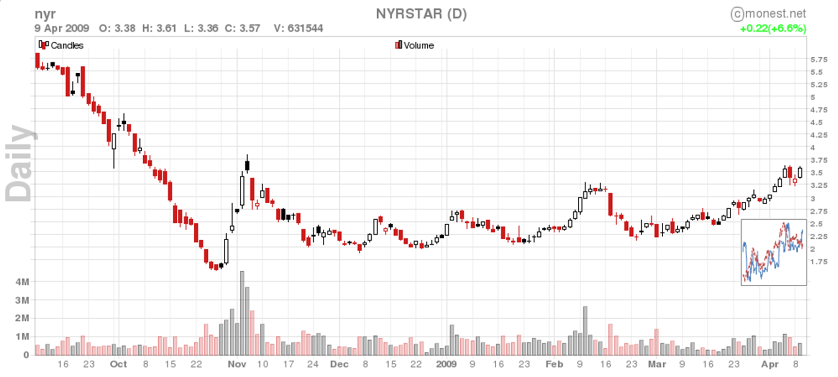Figure 1: This chart shows price action near the technically important level of €3.25. Beneath that particular zone, a small picture in picture box shows the effective volume around that time, calculated from the previous two weeks worth of transactions. [SOURCE] www.chartmill.com

Effective Volume split in small/large volume/players.

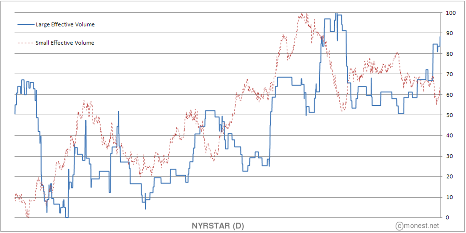Figure 2: This image is actually an enlargement of the picture-in—picture box of figure 1. Here it’s crystal clear that large volume/players is/are carrying the breakout while small players even seem to hand over their shares. Note that both indicators were rescaled to the [0, 100] interval.

Final Effective Volume implementation on ChartMill

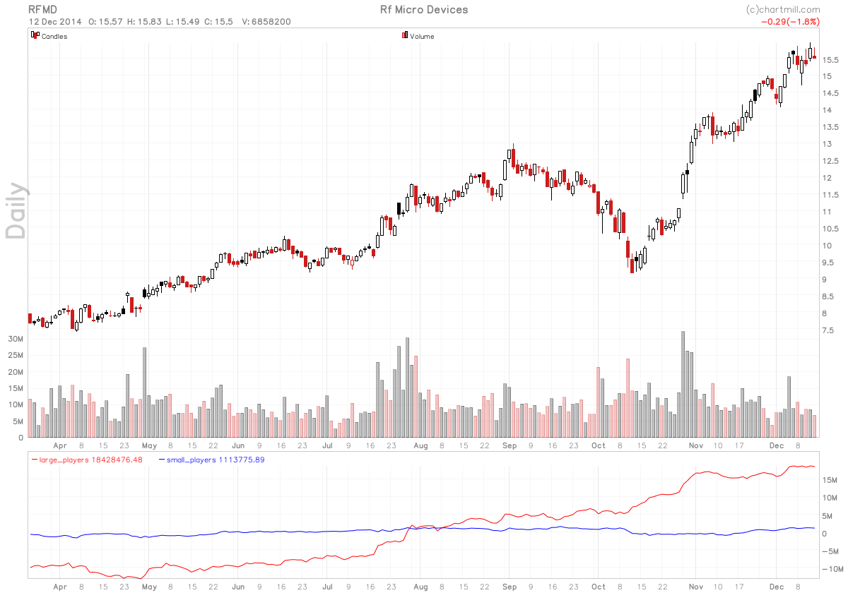Figure 3: Watch how large players effective volume accumulation is growing, while small players accumulation and distribution is holding ground. Although it would still be hard to trade short term, it definitely shows a longer term basis for a strong trend (as was the case in this example).